Quantum Espresso Workflow

This notebook builds the Quantum Espresso energy-volume-curve workflow with pyironflow.

An energy-volume curve is a standard calculation in computational materials science. The total energy of a crystal is computed for a series of volumes around the equilibrium volume. The minimum of the curve gives the equilibrium volume, and its curvature is related to the bulk modulus. Here, the curve is calculated for face-centered cubic aluminium with the density functional theory code Quantum ESPRESSO.

The workflow uses the following Python functions, defined in workflow.py:

Function	Purpose
get_bulk_structure	Build the cubic fcc aluminium unit cell (lattice constant a = 4.04 Å) with ASE.
calculate_qe	Write the input file for pw.x with ASE, run Quantum ESPRESSO, and parse the XML output. Returns the final structure, the energy and the volume.
generate_structures	Apply a list of volumetric strains to a structure. The cell is scaled by strain ** (1/3), so the volume changes by the factor strain.
plot_energy_volume_curve	Plot the energy as a function of the volume and save the figure as evcurve.png.

The workflow runs these steps in order:

1. Create the initial aluminium structure.

2. Relax the cell with a variable-cell relaxation (vc-relax) in Quantum ESPRESSO.

3. Generate five strained structures from the relaxed structure, with volumes between 90 % and 110 % of the relaxed volume.

4. Compute the total energy of each strained structure with a self-consistent field (scf) calculation. These five calculations are independent of each other, so a workflow engine can run them in parallel.

5. Collect the volumes and energies and plot the energy-volume curve.

Atomic structures are passed between the functions as JSON strings, using the OPTIMADE structure format, rather than as Python objects. This keeps the data exchanged between nodes serializable and independent of any particular workflow engine. The pseudopotential Al.pbe-n-kjpaw_psl.1.0.0.UPF used by Quantum ESPRESSO is provided in the espresso/pseudo directory.

The same workflow is implemented with other workflow engines in the Python Workflow Definition repository. This notebook first reloads the existing workflow.json in pyironflow and runs it. It then shows how the workflow is defined with pyiron_workflow and exported to workflow.json.

Reload workflow in pyironflow

load_workflow_json() reads workflow.json and builds a pyiron_workflow Workflow. Besides the functions from workflow.py, the JSON file refers to two helper functions that the Python Workflow Definition provides for all workflow engines:

• python_workflow_definition.shared.get_dict bundles several inputs into one dictionary. Here it builds the input_dict for each calculate_qe call from the structure, pseudopotentials, k-points, calculation type and smearing.

• python_workflow_definition.shared.get_list collects several inputs into one list. Here it gathers the five volumes and the five energies for the final plot.

These helpers appear as regular nodes in the pyironflow graph.

workflow_json_filename = "workflow.json"

from python_workflow_definition.pyiron_workflow import load_workflow_json

from pyironflow import PyironFlow

wf = load_workflow_json(file_name=workflow_json_filename)
PyironFlow([wf]).gui

The pyironflow interface is an interactive Jupyter widget, so it only appears in a live Jupyter session. The screenshot below shows the Quantum ESPRESSO workflow in pyironflow after it has been executed:

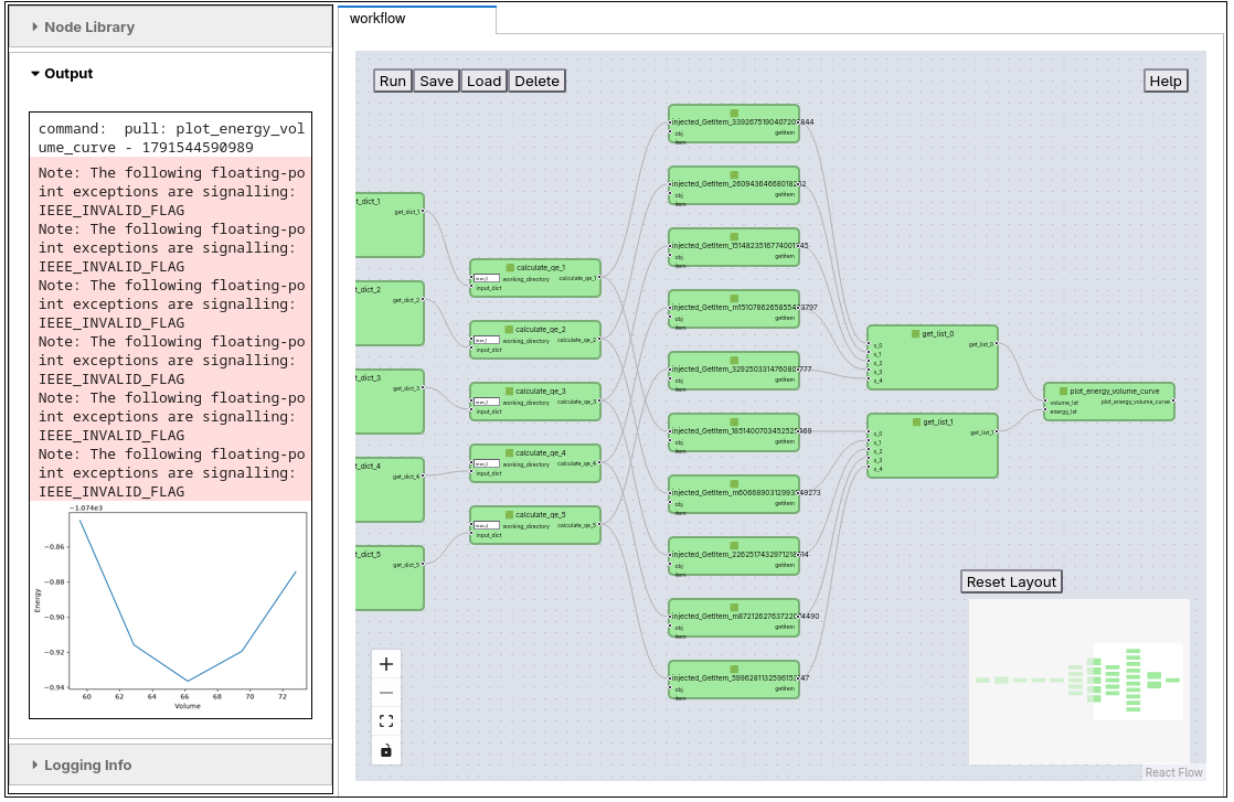
The user interface of pyironflow is split into two parts:

• Sidebar (left):

  • Node Library lists Python functions that can be added to the workflow as new nodes.

  • Output shows the result of the most recent execution, including anything the Python functions print to stdout or stderr.

  • Logging Info collects log messages of the workflow engine.

• Canvas (right): each workflow is shown in its own tab. The buttons in the top left are Run (execute the whole workflow), Save and Load (write the workflow, including its results, to storage and read it back) and Delete (remove the saved copy from storage). The controls in the bottom left zoom and fit the view. The Reset Layout button arranges the nodes automatically, and the minimap below it helps you find your way around larger graphs.

Each green box is a node, which is one Python function. Its input ports are on the left and its output ports on the right. Input values that do not come from another node can be edited in the fields next to the input ports. The lines between nodes are the edges of the workflow and show how data flows from one function to the next.

Besides running the whole workflow, you can work with individual nodes:

• Pull runs a node together with all upstream nodes it depends on.

• Push runs a node and all downstream nodes that depend on it.

• Reset clears the cached results of a node.

• The right-click menu offers View Output, which shows a node’s outputs without running it, and View Source, which shows the Python source code behind the node.

These options make it easy to inspect intermediate results while debugging a workflow.

The screenshot shows the right-hand part of the graph, where the five strained calculations fan out and are collected again. From left to right:

• get_dict_1 to get_dict_5 build the input dictionaries for the five strained structures.

• calculate_qe_1 to calculate_qe_5 run the scf calculations.

• Pairs of injected_GetItem nodes extract the energy and the volume from each result dictionary.

• get_list_0 and get_list_1 collect the volumes and the energies into two lists.

• plot_energy_volume_curve produces the final plot.

The initial structure, the vc-relax calculation and generate_structures are further to the left, as shown in the minimap. A graph like this shows the parallel structure of the workflow at a glance, which is much harder to see in the JSON file.

The Output panel shows the result of pulling the plot_energy_volume_curve node. The resulting energy-volume curve has its minimum close to the volume of the relaxed structure. The red notes about IEEE_INVALID_FLAG are printed by the Fortran runtime when pw.x exits, once for each of the six Quantum ESPRESSO calculations. They are informational and do not mean the calculations failed.

wf.run()

Note: The following floating-point exceptions are signalling: IEEE_INVALID_FLAG
Note: The following floating-point exceptions are signalling: IEEE_INVALID_FLAG
Note: The following floating-point exceptions are signalling: IEEE_INVALID_FLAG
Note: The following floating-point exceptions are signalling: IEEE_INVALID_FLAG
Note: The following floating-point exceptions are signalling: IEEE_INVALID_FLAG
Note: The following floating-point exceptions are signalling: IEEE_INVALID_FLAG

{'plot_energy_volume_curve__plot_energy_volume_curve': <Figure size 640x480 with 1 Axes>}

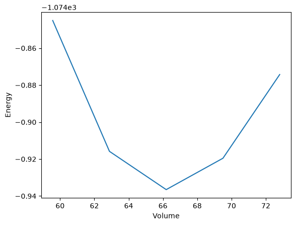
wf.run() runs the same workflow from Python. It performs one vc-relax and five scf calculations with Quantum ESPRESSO, in the working directories mini and strain_0 to strain_4, and returns the matplotlib figure of the energy-volume curve. The figure is also saved as evcurve.png.

Define workflow with pyiron_workflow

This part shows how workflow.json was created. pyironflow is a graphical front end for pyiron_workflow, so the workflow is defined with the pyiron_workflow Python interface.

Plain functions are converted to graph nodes with to_function_node, assembled into a Workflow via attribute access, and exported as a PWD workflow.json.

from inspect import isfunction
import numpy as np
from pyiron_workflow import Workflow, to_function_node, as_function_node
from pyiron_workflow.api import inputs_to_dict
from python_workflow_definition.pyiron_workflow import write_workflow_json

from workflow import (
    calculate_qe as _calculate_qe, 
    generate_structures as _generate_structures, 
    get_bulk_structure as _get_bulk_structure, 
    plot_energy_volume_curve as _plot_energy_volume_curve,
)

pyiron_workflow has no built-in equivalent of the get_list helper the other engines use to collect several outputs into a list, so get_values_from_dict is defined here as a custom node with as_function_node to turn a dict of energies/volumes into a plain list for the final plot.

@as_function_node("output_dict")
def get_values_from_dict(input_dict):
    return list(input_dict.values())

calculate_qe = to_function_node("calculate_qe", _calculate_qe, "calculate_qe")
generate_structures = to_function_node("generate_structures", _generate_structures, "generate_structures")
get_bulk_structure = to_function_node("get_bulk_structure", _get_bulk_structure, "get_bulk_structure")
plot_energy_volume_curve = to_function_node("plot_energy_volume_curve", _plot_energy_volume_curve, "plot_energy_volume_curve", validate_output_labels=False)

to_function_node wraps each plain Python function into a pyiron_workflow node type. plot_energy_volume_curve passes validate_output_labels=False since it has no return value, so its output cannot be matched to an explicit output label.

wf = Workflow("my_workflow")

The pseudopotentials are defined once as a workflow-level value. All six Quantum ESPRESSO calculations use the same value, so it appears as a single input node in the exported workflow.json.

wf.pseudopotentials = {"Al": "Al.pbe-n-kjpaw_psl.1.0.0.UPF"}

Nodes are added to the Workflow by assigning their result to an attribute of wf (e.g. wf.structure = get_bulk_structure(...)), which both registers the node and gives it a name in the graph. Since calculate_qe expects a single input_dict argument, inputs_to_dict is used to bundle the structure, pseudopotentials, k-points, calculation type and smearing into one dict-valued node before the first (vc-relax) QE calculation.

wf.element = "Al"
wf.a = 4.04
wf.cubic = True
wf.structure = get_bulk_structure(
    element=wf.element,
    a=wf.a,
    cubic=wf.cubic,
)

wf.working_directory_0 = "mini"
input_dict = {
    "structure": wf.structure, 
    "pseudopotentials": wf.pseudopotentials, 
    "kpts": (3, 3, 3), 
    "calculation": "vc-relax", 
    "smearing": 0.02,
}
wf.input_dict_0 = inputs_to_dict(
    input_specification=list(input_dict.keys()),
    **input_dict
)

The first calculate_qe node runs the variable-cell relaxation in the working directory mini. Its output dictionary contains the relaxed structure, which is the starting point for the strained structures.

wf.calc_mini = calculate_qe(
    working_directory=wf.working_directory_0,
    input_dict=wf.input_dict_0,
)

generate_structures fans out the relaxed structure into number_of_strains (5) strained structures (wf.structure_lst["s_0"] … ["s_4"]). The loop below builds one input_dict and one independent scf calculate_qe node per strained structure, so five QE calculations run to sample the energy-volume curve.

number_of_strains = 5
wf.strain_lst = np.linspace(0.9, 1.1, number_of_strains)
wf.structure_lst = generate_structures(  # the generate_structures() function is not available in the workflow graph
    structure=wf.calc_mini["structure"],
    strain_lst=wf.strain_lst,
)

job_strain_lst = []
for i in range(number_of_strains):
    setattr(wf, "input_dict_" + str(i+1), inputs_to_dict(
        input_specification=["structure", "pseudopotentials", "kpts", "calculation", "smearing"],
        structure=wf.structure_lst["s_" + str(i)],
        pseudopotentials=wf.pseudopotentials,
        kpts=(3, 3, 3),
        calculation="scf",
        smearing=0.02,
    ))
    setattr(wf, "calc_strain_" + str(i), calculate_qe(
        working_directory="strain_" + str(i),
        input_dict=getattr(wf, "input_dict_" + str(i+1)),
    ))
    job_strain_lst.append(getattr(wf, "calc_strain_" + str(i)))

The energy and volume outputs of the five strained calculations are bundled with inputs_to_dict and then flattened into two plain lists with the get_values_from_dict node defined above, ready to be passed to plot_energy_volume_curve.

volume_dict = {"s_" + str(i): j["volume"] for i, j in enumerate(job_strain_lst)}
wf.volume_dict = inputs_to_dict(
    input_specification=list(volume_dict.keys()),
    **volume_dict
)
energy_dict = {"s_" + str(i): j["energy"] for i, j in enumerate(job_strain_lst)}
wf.energy_dict = inputs_to_dict(
    input_specification=list(energy_dict.keys()),
    **energy_dict,
)
wf.volume_lst = get_values_from_dict(
    input_dict=wf.volume_dict
)
wf.energy_lst = get_values_from_dict(
    input_dict=wf.energy_dict
)

Finally, the two lists are passed to plot_energy_volume_curve, which produces the last node of the workflow.

wf.plot = plot_energy_volume_curve(volume_lst=wf.volume_lst, energy_lst=wf.energy_lst)

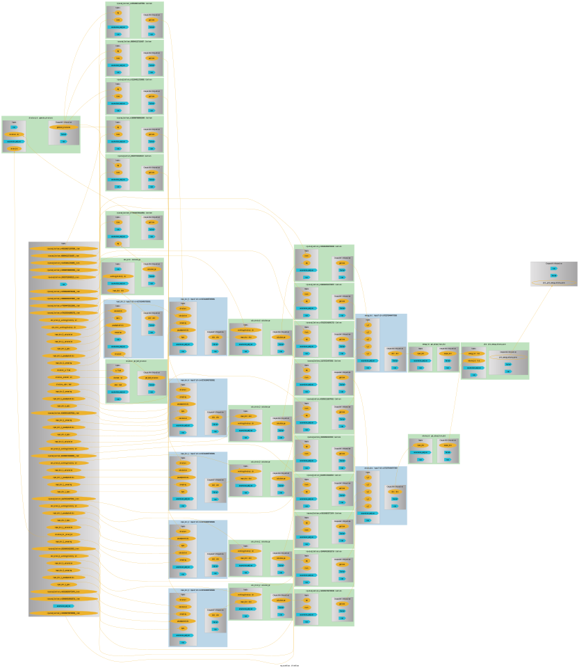
.draw() renders the assembled node graph, and write_workflow_json exports it - using wf.graph_as_dict - to the PWD workflow.json format so it can be loaded by another engine.

wf.draw(size=(10,10))

write_workflow_json(graph_as_dict=wf.graph_as_dict, file_name=workflow_json_filename)

!cat {workflow_json_filename}

{
  "version": "0.1.0",
  "nodes": [
    {
      "id": 0,
      "type": "function",
      "value": "workflow.get_bulk_structure"
    },
    {
      "id": 1,
      "type": "function",
      "value": "python_workflow_definition.shared.get_dict"
    },
    {
      "id": 2,
      "type": "function",
      "value": "workflow.calculate_qe"
    },
    {
      "id": 3,
      "type": "function",
      "value": "workflow.generate_structures"
    },
    {
      "id": 4,
      "type": "function",
      "value": "python_workflow_definition.shared.get_dict"
    },
    {
      "id": 5,
      "type": "function",
      "value": "workflow.calculate_qe"
    },
    {
      "id": 6,
      "type": "function",
      "value": "python_workflow_definition.shared.get_dict"
    },
    {
      "id": 7,
      "type": "function",
      "value": "workflow.calculate_qe"
    },
    {
      "id": 8,
      "type": "function",
      "value": "python_workflow_definition.shared.get_dict"
    },
    {
      "id": 9,
      "type": "function",
      "value": "workflow.calculate_qe"
    },
    {
      "id": 10,
      "type": "function",
      "value": "python_workflow_definition.shared.get_dict"
    },
    {
      "id": 11,
      "type": "function",
      "value": "workflow.calculate_qe"
    },
    {
      "id": 12,
      "type": "function",
      "value": "python_workflow_definition.shared.get_dict"
    },
    {
      "id": 13,
      "type": "function",
      "value": "workflow.calculate_qe"
    },
    {
      "id": 14,
      "type": "function",
      "value": "python_workflow_definition.shared.get_list"
    },
    {
      "id": 15,
      "type": "function",
      "value": "python_workflow_definition.shared.get_list"
    },
    {
      "id": 16,
      "type": "function",
      "value": "workflow.plot_energy_volume_curve"
    },
    {
      "id": 17,
      "type": "input",
      "name": "element",
      "value": "Al"
    },
    {
      "id": 18,
      "type": "input",
      "name": "a",
      "value": 4.04
    },
    {
      "id": 19,
      "type": "input",
      "name": "cubic",
      "value": true
    },
    {
      "id": 20,
      "type": "input",
      "name": "pseudopotentials",
      "value": {
        "Al": "Al.pbe-n-kjpaw_psl.1.0.0.UPF"
      }
    },
    {
      "id": 21,
      "type": "input",
      "name": "kpts",
      "value": [
        3,
        3,
        3
      ]
    },
    {
      "id": 22,
      "type": "input",
      "name": "calculation_0",
      "value": "vc-relax"
    },
    {
      "id": 23,
      "type": "input",
      "name": "smearing",
      "value": 0.02
    },
    {
      "id": 24,
      "type": "input",
      "name": "working_directory_0",
      "value": "mini"
    },
    {
      "id": 25,
      "type": "input",
      "name": "strain_lst",
      "value": [
        0.9,
        0.9500000000000001,
        1.0,
        1.05,
        1.1
      ]
    },
    {
      "id": 26,
      "type": "input",
      "name": "calculation_1",
      "value": "scf"
    },
    {
      "id": 27,
      "type": "input",
      "name": "working_directory_1",
      "value": "strain_0"
    },
    {
      "id": 28,
      "type": "input",
      "name": "working_directory_2",
      "value": "strain_1"
    },
    {
      "id": 29,
      "type": "input",
      "name": "working_directory_3",
      "value": "strain_2"
    },
    {
      "id": 30,
      "type": "input",
      "name": "working_directory_4",
      "value": "strain_3"
    },
    {
      "id": 31,
      "type": "input",
      "name": "working_directory_5",
      "value": "strain_4"
    },
    {
      "id": 32,
      "type": "output",
      "name": "result"
    }
  ],
  "edges": [
    {
      "target": 3,
      "targetPort": "structure",
      "source": 2,
      "sourcePort": "structure"
    },
    {
      "target": 12,
      "targetPort": "structure",
      "source": 3,
      "sourcePort": "s_4"
    },
    {
      "target": 10,
      "targetPort": "structure",
      "source": 3,
      "sourcePort": "s_3"
    },
    {
      "target": 8,
      "targetPort": "structure",
      "source": 3,
      "sourcePort": "s_2"
    },
    {
      "target": 6,
      "targetPort": "structure",
      "source": 3,
      "sourcePort": "s_1"
    },
    {
      "target": 4,
      "targetPort": "structure",
      "source": 3,
      "sourcePort": "s_0"
    },
    {
      "target": 15,
      "targetPort": "0",
      "source": 5,
      "sourcePort": "energy"
    },
    {
      "target": 14,
      "targetPort": "0",
      "source": 5,
      "sourcePort": "volume"
    },
    {
      "target": 15,
      "targetPort": "1",
      "source": 7,
      "sourcePort": "energy"
    },
    {
      "target": 14,
      "targetPort": "1",
      "source": 7,
      "sourcePort": "volume"
    },
    {
      "target": 15,
      "targetPort": "2",
      "source": 9,
      "sourcePort": "energy"
    },
    {
      "target": 14,
      "targetPort": "2",
      "source": 9,
      "sourcePort": "volume"
    },
    {
      "target": 15,
      "targetPort": "3",
      "source": 11,
      "sourcePort": "energy"
    },
    {
      "target": 14,
      "targetPort": "3",
      "source": 11,
      "sourcePort": "volume"
    },
    {
      "target": 15,
      "targetPort": "4",
      "source": 13,
      "sourcePort": "energy"
    },
    {
      "target": 14,
      "targetPort": "4",
      "source": 13,
      "sourcePort": "volume"
    },
    {
      "target": 1,
      "targetPort": "structure",
      "source": 0,
      "sourcePort": null
    },
    {
      "target": 2,
      "targetPort": "input_dict",
      "source": 1,
      "sourcePort": null
    },
    {
      "target": 5,
      "targetPort": "input_dict",
      "source": 4,
      "sourcePort": null
    },
    {
      "target": 7,
      "targetPort": "input_dict",
      "source": 6,
      "sourcePort": null
    },
    {
      "target": 9,
      "targetPort": "input_dict",
      "source": 8,
      "sourcePort": null
    },
    {
      "target": 11,
      "targetPort": "input_dict",
      "source": 10,
      "sourcePort": null
    },
    {
      "target": 13,
      "targetPort": "input_dict",
      "source": 12,
      "sourcePort": null
    },
    {
      "target": 16,
      "targetPort": "volume_lst",
      "source": 14,
      "sourcePort": null
    },
    {
      "target": 16,
      "targetPort": "energy_lst",
      "source": 15,
      "sourcePort": null
    },
    {
      "target": 0,
      "targetPort": "element",
      "source": 17,
      "sourcePort": null
    },
    {
      "target": 0,
      "targetPort": "a",
      "source": 18,
      "sourcePort": null
    },
    {
      "target": 0,
      "targetPort": "cubic",
      "source": 19,
      "sourcePort": null
    },
    {
      "target": 1,
      "targetPort": "pseudopotentials",
      "source": 20,
      "sourcePort": null
    },
    {
      "target": 1,
      "targetPort": "kpts",
      "source": 21,
      "sourcePort": null
    },
    {
      "target": 1,
      "targetPort": "calculation",
      "source": 22,
      "sourcePort": null
    },
    {
      "target": 1,
      "targetPort": "smearing",
      "source": 23,
      "sourcePort": null
    },
    {
      "target": 2,
      "targetPort": "working_directory",
      "source": 24,
      "sourcePort": null
    },
    {
      "target": 3,
      "targetPort": "strain_lst",
      "source": 25,
      "sourcePort": null
    },
    {
      "target": 4,
      "targetPort": "pseudopotentials",
      "source": 20,
      "sourcePort": null
    },
    {
      "target": 4,
      "targetPort": "kpts",
      "source": 21,
      "sourcePort": null
    },
    {
      "target": 4,
      "targetPort": "calculation",
      "source": 26,
      "sourcePort": null
    },
    {
      "target": 4,
      "targetPort": "smearing",
      "source": 23,
      "sourcePort": null
    },
    {
      "target": 5,
      "targetPort": "working_directory",
      "source": 27,
      "sourcePort": null
    },
    {
      "target": 6,
      "targetPort": "pseudopotentials",
      "source": 20,
      "sourcePort": null
    },
    {
      "target": 6,
      "targetPort": "kpts",
      "source": 21,
      "sourcePort": null
    },
    {
      "target": 6,
      "targetPort": "calculation",
      "source": 26,
      "sourcePort": null
    },
    {
      "target": 6,
      "targetPort": "smearing",
      "source": 23,
      "sourcePort": null
    },
    {
      "target": 7,
      "targetPort": "working_directory",
      "source": 28,
      "sourcePort": null
    },
    {
      "target": 8,
      "targetPort": "pseudopotentials",
      "source": 20,
      "sourcePort": null
    },
    {
      "target": 8,
      "targetPort": "kpts",
      "source": 21,
      "sourcePort": null
    },
    {
      "target": 8,
      "targetPort": "calculation",
      "source": 26,
      "sourcePort": null
    },
    {
      "target": 8,
      "targetPort": "smearing",
      "source": 23,
      "sourcePort": null
    },
    {
      "target": 9,
      "targetPort": "working_directory",
      "source": 29,
      "sourcePort": null
    },
    {
      "target": 10,
      "targetPort": "pseudopotentials",
      "source": 20,
      "sourcePort": null
    },
    {
      "target": 10,
      "targetPort": "kpts",
      "source": 21,
      "sourcePort": null
    },
    {
      "target": 10,
      "targetPort": "calculation",
      "source": 26,
      "sourcePort": null
    },
    {
      "target": 10,
      "targetPort": "smearing",
      "source": 23,
      "sourcePort": null
    },
    {
      "target": 11,
      "targetPort": "working_directory",
      "source": 30,
      "sourcePort": null
    },
    {
      "target": 12,
      "targetPort": "pseudopotentials",
      "source": 20,
      "sourcePort": null
    },
    {
      "target": 12,
      "targetPort": "kpts",
      "source": 21,
      "sourcePort": null
    },
    {
      "target": 12,
      "targetPort": "calculation",
      "source": 26,
      "sourcePort": null
    },
    {
      "target": 12,
      "targetPort": "smearing",
      "source": 23,
      "sourcePort": null
    },
    {
      "target": 13,
      "targetPort": "working_directory",
      "source": 31,
      "sourcePort": null
    },
    {
      "target": 32,
      "targetPort": null,
      "source": 16,
      "sourcePort": null
    }
  ]
}

The exported workflow.json contains 17 function nodes, 15 input nodes and one output node:

• Function nodes: get_bulk_structure, six get_dict and six calculate_qe nodes (one each for the relaxation and the five strained structures), generate_structures, two get_list nodes and plot_energy_volume_curve.

• Input nodes: each distinct input value appears once. pseudopotentials, kpts and smearing are shared by all six get_dict nodes. The two calculation types are stored as calculation_0 (vc-relax) and calculation_1 (scf). The six working directories are stored as working_directory_0 to working_directory_5.

• Engine-specific helpers: the pyiron_workflow nodes inputs_to_dict and get_values_from_dict used above are not part of the file. They are replaced by the engine-independent helpers python_workflow_definition.shared.get_dict and get_list. This is why the reloaded workflow in the first part of this notebook contains get_dict and get_list nodes.

With this translation, the same workflow.json can be executed with any workflow engine supported by the Python Workflow Definition, or explored visually with pyironflow.